文章目录
一、概述
1.1 常量传播
常量传播(constant propagation)是一种转换,对于给定的关于某个变量 x x x和一个常量 c c c的赋值 x ← c x\leftarrow c x←c,这种转换用 c c c来替代以后出现的 x x x的引用,只要在这期间没有出现另外改变 x x x值的赋值。
如下图a的CFG所示,基本块B1中的指令
b
←
3
b\leftarrow 3
b←3将常量3赋给
b
b
b,并且CFG中没有其他对
b
b
b的赋值。图b是对图a做常量传播的结果,此时
b
b
b的所有出现都已被3替换,但都没有对结果得到的常数表达式进行计算(就是常量折叠,这里也可以直接结算)。
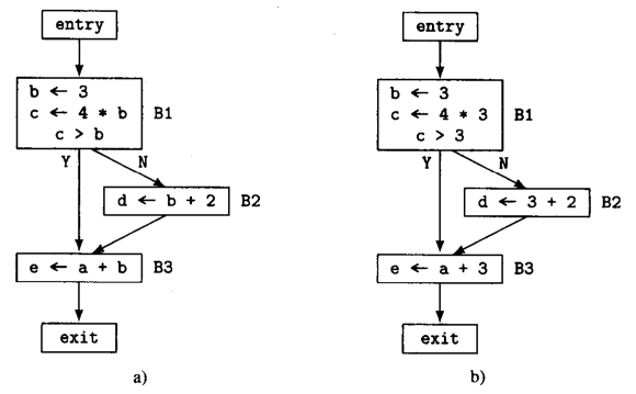
正是因为常量传播的优化操作,使得指令
b
←
3
b\leftarrow 3
b←3成为无用代码(没有在其他的指令操作数中引用),死代码删除时可以将
b
←
3
b\leftarrow 3
b←3删除。
1.2 SSCP 和 SCCP的区别
在《编译器设计》总结中介绍过稀疏简单常量传播(Sparse Simple Constant Propagation,SSCP),这里将要介绍的是稀疏条件常量传播(Sparse Conditional Constant Propagation,SCCP),它和SSCP实现方法相似,只是传播方式不同,两者在CFG中处理常量传播时的主要区别如下:
- 传播方式。SCCP的常量值只沿着可达的控制流路径传播,当遇到条件分支时,只有符合条件的路径上的常量值才会被传播;SSCP则是一种更为简单的常量传播方法,它不考虑控制流条件,而是在整个控制流图中的所有路径上进行常量传播。
- 传播精度。SCCP由于只在符合条件的控制流路径上传播常量,因此稀疏条件常量传播的精度相对较高。它能够更准确地确定哪些值可以在运行时被计算为常量。SSCP稀疏简单常量传播的精度相对较低,因为它忽略了条件分支,常常会导致在一些路径上的常量传播不正确。
- 复杂度。SCCP由于考虑了控制流条件,稀疏条件常量传播的算法复杂度相对较高,但它更准确。SSCP稀疏简单常量传播的算法相对简单,但它的精度较低,可能会导致一些常量传播的机会被忽略。
1.3 Golang中SCCP不完善点
目前主要存在以下几个不完善点:
- 尚不支持nil和string常量的传播。
- 只支持函数内部常量传播,尚不支持过程间的传播。
- SCCP和prove等pass存在重复优化,其实是可以整合一下的。
- 最后一个是Phi的
top ∩ constant = constant的设计,在我的理解上改成top ∩ constant = top更好,但我不确定这样是否会引入问题,以后看看其他编译器的实现再来考究。
二、稀疏条件常量传播
Golang中关于SCCP的实现在文件src/cmd/compile/internal/ssa/sccp.go中,算法的开始函数是sccp(f *Func) 函数。SCCP算法实现的步骤主要分为:
- 初始化
worklist: 首先,需要初始化worklist中存放的必要数据结构,以便记录控制流图、变量的使用情况和 lattice 等信息。 - 构建
def-use链: 遍历函数的基本块和值,构建每个值的def-use链,以确定哪些值的常量可以被传播。 - 传播常量: 遍历每个基本块和其中的Value,对每个Value应用稀疏条件常量传播算法。这包括检查Value的操作类型,确定其是否可以被折叠为常量,并根据参数更新
lattice。对于具有多个后继的基本块,根据控制Value的lattice更新传播路径。 - 重写no-constant: 一旦确定了可以替换为常量的值,将其替换为相应的常量。同时,更新相应基本块的控制流以反映这些常量值的传播。
以下是我提取的 SSA IR 代码片段。接下来,将详细介绍 SCCP 算法的实现步骤,并在解释过程中引入这段代码,以帮助理解。
b1:
    v1 = InitMem <mem>
    v5 = Const64 <int> [0]
    v6 = Const64 <int> [1]
    v7 = Const64 <int> [2]
    v8 = Const64 <int> [3]
    v9 = Add64 <int> v8 v7
    v10 = Less64 <bool> v5 v6
If v10 → b3 b2

b3: ← b1
    v13 = Add64 <int> v6 v7
Plain → b2

b2: ← b1 b3
    v19 = Phi <int> v9 v13
    v16 = Add64 <int> v6 v7
    v18 = Add64 <int> v7 v8
    v20 = Add64 <int> v19 v16
    v21 = Add64 <int> v20 v18
    v23 = MakeResult <int,mem> v21 v1
Ret v23
2.1 初始化worklist
worklist是一个存放多种数据结构的集合,也可以认为是SCCP算法的上下文,其结构定义如下:
type worklist struct {
	f            *Func               // 当前正在优化的函数
	edges        []Edge              // 传播时遍历CFG的edge队列,广度优先遍历
	uses         []*Value            // 当一个值的lattice改变时,将其使用链append其中
	visited      map[Edge]bool       // 记录一条edge是否传播过
	latticeCells map[*Value]lattice  // 值的lattice,传播过程会更新
	defUse       map[*Value][]*Value // 非控制值的def-use链
	defBlock     map[*Value][]*Block // 控制值的def-use链,控制值只在个别块中使用
	visitedBlock []bool              // 记录一个block是否访问过
}
初始化worklist就是初始化worklist中的数据结构,如上代码块。需要注意defUse和defBlock,其map的key是Value对象,map的value是个一维数组。
2.2 构建def-use链
def-use链是指Value的定义和使用之间的关系链,对任意一个Value的定义,都可以通过def-use链找到所有使用该Value的目标(以该Value为参数的Value)。如IR片段中的定义v6,使用过v6的Value有v10,v13和v16,所以defUse[v6] = {v10, v13, v16}。控制Value的定义,对应的使用都是Block。如IR片段中的定义v10,使用v10的Block有If,所以defBlock[v10] = {If}
这里不需要为所有的Value构建def-use链,而只为可能为常量(lattice为top或constant) 的Value构建。因为对于不可能是常量(lattice为bottom) 的Value,不管其lattice更新多少次,都会保持bottom不变。构建规则如下:
- 如果一个Value
v1的定义可能为常量,且引用v1的Valuev2也可能为常量,则将v2加入到v1的def-use链defUse[v1]中; - 如果一个Value
v1的定义可能为常量,但引用v1的Valuev2不可能是常量,则不能将v2加入到v1的def-use链defUse[v1]中; - 如果一个Value
v1的定义不可能是常量,则不用构建v1的def-use链defUse[v1]。
检测一个Value是否可能为常量由possibleConst函数实现。如果一个Value的opcode是常量操作(ConstBool、ConstString、ConstNil、Const8等),那么该Value肯定就是一个常量。如果一个Value的opcode能够满足,一旦操作数是常量,其结果肯定就是常量,那么该Value可能就是一个常量。这类opcode有算数运算、位运算、比较、转换等。
构建def-use链的过程,在buildDefUses函数中实现。其主要逻辑如下:
- 遍历函数的Block。
- 遍历Block的Value的定义
val。
如果val与其参数arg满足上文构建规则1,则将val加入到arg对应的def-use链中,即t.defUse[arg] = append(t.defUse[arg], val)。 - 遍历Block的控制Value
ctl。
如果ctl可能是常量,则将当前块加入到ctl对应的def-use链中,即t.defBlock[ctl] = append(t.defBlock[ctl], block)。
- 遍历Block的Value的定义
构建IR片段def-use链,Value和控制Value分别得到的defUse和defBlock分别如下:
defUse = map[*Value][]*Value {
    //def   use
    v5:     {v10},
    v6:     {v10,v13,v16},
    v7:     {v9,v13,v16,v18},
    v8:     {v9,v18},
    v9:     {v19},
    v13:    {v19},
    v19:    {v20},
    v16:    {v20},
    v18:    {v21},
    v20:    {v21},
	// v1不可能是常量
}

defBlock = map[*Value][]*Block {
    //def	use
    v10:	{If},
	// v23不可能是常量
}
2.3 传播constant
SCCP给函数的每个Value都设置了一个lattice,根据lattice->tag的值可以知道一个Value可能是常量(top)、是常量(constant) 或者 不可能是常量(bottom)。Value与其lattice的对应关系存放在worklist->latticeCells中,该结构是个map,key是Value对象,value是Value的lattice对象。
SCCP算法最初,将所有可能是常量的Value的lattice认为是top,所有确定不是常量的Value的lattice认为是bot。IR片段中各个Value的初始lattice如下:
latticeCells = map[*Value]lattice {
    v1:     lattice{bottom, nil},
    v5:     lattice{top, nil},
    v6:     lattice{top, nil},
    v7:     lattice{top, nil},
    v8:     lattice{top, nil},
    v9:     lattice{top, nil},
    v10:    lattice{top, nil},
    v13:    lattice{top, nil},
    v16:    lattice{top, nil},
    v18:    lattice{top, nil},
    v19:    lattice{top, nil},
    v20:    lattice{top, nil},
    v21:    lattice{top, nil},
    v23:    lattice{bottom, nil},
}
构建def-use链完成之后,从函数的entry Block开始,广度优先遍历CFG,访问每个Block上的Value,其目的是更新Value的lattice。访问Value在函数visitValue中实现,如果一个Value的lattice在访问过程中发生了变化,则执行addUses函数,将该Value定义对应def-use链上的所有使用,加入到worklist->uses中。最后遍历worklist->uses,直至所有Value的lattice都不再更新为止。
所谓更新Value的lattice,其实就是确定一个可能是常量 的Value到底是常量 还是非常量 的过程,对应到lattice就是lattice->tag由top转变为constant或bottom,Phi指令还会从constant转变为bottom。
为了方便计算更新各个指令结果Value的lattice,将可能为常量的指令划分为以下5类。除了常量指令外,其余指令结果Value的lattice都要根据参数的lattice来计算。如下所示:
-
常量指令。Value的Opcode为
ConstXX,表示其是一个常量指令。这类Value我们已经确定其是常量,不用分析参数,直接指定lattice为{constant, const_val}即可。 -
Copy指令。该指令不做运算,只是对
Arg[0]的复制,所以其结果Value的lattice完全依赖于Args[0]的lattice。 -
Phi指令。该指令结果Value的lattice,使用了半格的meet运算规则来降级,对应的
latticemeet运算规则如下:Top ∩ any = any Bottom ∩ any = Bottom ConstantA ∩ ConstantA = ConstantA ConstantA ∩ ConstantB = BottomPhi的参数只要有一个是
bottom,则其结果为bottom。
Phi参数如果都为constant,有且仅有所有参数的常量值都相等时,结果才会为一个与参数相等的常量值,其余情况均为bottom。
Phi参数如果top与constant共存,结果即可以保持top不变,也可以降为constant。作者采用了后者,top ∩ constant = constant,这样Phi结果Value的lattice就会有更新两次的情况,如下:- 1)如果top参数最终降级为constant,且与其他常量参数的值相等,Phi结果Value的lattice只经过了top => constant。
- 2)如果top参数最终降为bottom,或者降为constan但常量值与其他参数不想等。此时结果Value的lattice要从constant变为bottom,所以Phi结果Value的lattice经过了top => constant => bottom。
我们可以在任何情况下,只让Phi结果Value的
lattice更新一次。top与constant共存时,让top ∩ constant = top,上面情况一 不变继续是top => constant,情况二 则是由top => constant => bottom变成top => bottom。少了一次降级,这样Phi结果Value的use链就少一次更新,从而提高传播速度。 -
一元运算指令。该指令对
Arg[0]做运算,所以其结果Value的lattice也是完全依赖于Args[0]的lattice。但如果Args[0]的lattice.tag=constant,即是常量,则要将Args[0]常量值带入该一元指令做运算,并将算出来的结果result_val设置到lattice{constant, result_val},这其实就是常量折叠,由函数computeLattice完成。 -
二元运算指令。该指令对
Arg[0]和Arg[1]两个参数做运算,同理其结果Value的lattice也是完全依赖于参数的lattice。如果两个参数均为常量,则进行常量折叠;如果有任意一个参数为非常量,则运算结果为非常量,即lattice为{bottom, nil};如果两个参数都不确定,则运算结果也不确定,lattice为{top, nil}。
待worklist->uses遍历完成,所有lattice不再更新。此时IR片段中各个Value的lattice如下:
latticeCells = map[*Value]lattice {
    v1:     lattice{bottom, nil},
    v5:     lattice{constant, 0},
    v6:     lattice{constant, 1},
    v7:     lattice{constant, 2},
    v8:     lattice{constant, 3},
    v9:     lattice{constant, 5},
    v10:    lattice{constant, 1},
    v13:    lattice{constant, 3},
    v16:    lattice{constant, 3},
    v18:    lattice{constant, 5},
    v19:    lattice{bottom, nil},
    v20:    lattice{bottom, nil},
    v21:    lattice{bottom, nil},
    v23:    lattice{bottom, nil},
}
2.4 重写no-constant
待所有Value的lattice更新完成后,就可以遍历worklist->latticeCells,根据worklist->latticeCells[Value].tag确定一个Value是常量还是非常量。
如果一个Value的lattice.tag=constant,但Value本身不是常量,说明该Value是经过SCCP确定的常量,我们要将其重写为常量Value;如果Value是控制Value,我们还要根据常量值Value.AuxInt,重写使用该控制Value的Block到其后继Block的边,即将不可达的一条边删除。删除一条边的方法在《Golang编译优化——死代码删除》中已经介绍过。
重写Value时应该将其参数Args置为nil(val.Args = nil),这样在死代码删除时才能发挥作用。IR片段重写no-constant后如下所示:
b1:
    v1 = InitMem <mem>
    v5 = Const64 <int> [0]
    v6 = Const64 <int> [1]
    v7 = Const64 <int> [2]
    v8 = Const64 <int> [3]
    v9 = Const64 <int> [5]
    v10 = Const64 [1]
Plain → b3

b3: ← b1
    v13 = Const64 <int> [3]
Plain → b2

b2: ← b1 b3
    v19 = Phi <int> v9 v13
    v16 = Const64 <int> [3]
    v18 = Const64 <int> [5]
    v20 = Add64 <int> v19 v16
    v21 = Add64 <int> v20 v18
    v23 = MakeResult <int,mem> v21 v1
Ret v23
重写完成以后,在后续的deadcode pass中,会将重写no-constant暴露出的死代码删除。关于死代码删除的pass,之前写文章总结过。如下是删除死代码后的IR片段:
b1:
    v1 = InitMem <mem>
    v9 = Const64 <int> [5]
Plain → b3

b3: ← b1
    v13 = Const64 <int> [3]
Plain → b2

b2: ← b3
    v19 = Phi <int> v9 v13
    v16 = Const64 <int> [3]
    v18 = Const64 <int> [5]
    v20 = Add64 <int> v19 v16
    v21 = Add64 <int> v20 v18
    v23 = MakeResult <int,mem> v21 v1
Ret v23
可以看出,上列代码并不是最好的优化代码。还可以有很多优化的点,这些优化点会在其他的pass中处理,如:
-
b2只有b3一个前趋Block,deadcode pass删除一条边时可以将v19 = Phi <int> v9 v13变成v19 = Copy <int> v13; - 通过复制传播将
v19 = Copy <int> v13消除,v20 = Add64 <int> v19 v16会变成v20 = Add64 <int> v19 v13; -
b1 -> b3,b3 -> b2可以通过fuse pass合并成一个基本块;